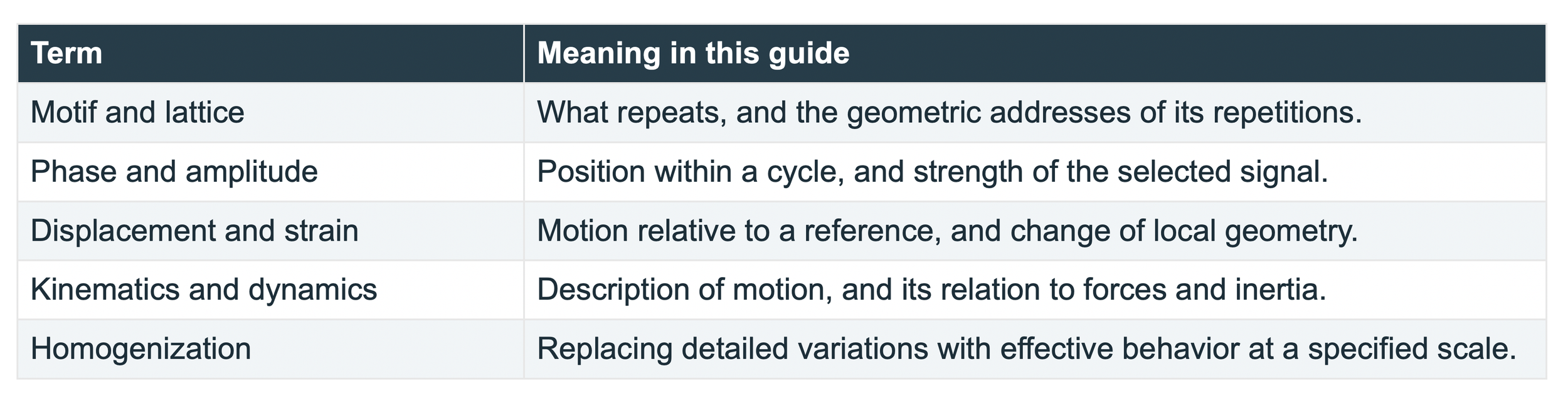
This article is a study guide for a paper titled: Determination of Displacement Fields at the Sub-Nanometric Scale (2019) by C. A. Sciammarella, F. M. Sciammarella, and L. Lamberti.
A crystal gives us a repeating pattern that can act as its own measuring ruler. When that pattern changes, digital moire analysis can recover tiny displacements and describe how neighboring regions stretch, rotate, or shear. A field map can reveal where deformation concentrates around a defect even when the whole specimen changes very little. This makes images a way to test the connection between atomic arrangements and the smooth fields used in engineering.
This guide explains the 2019 paper by Cesar A. Sciammarella, Federico M. Sciammarella, and Luciano Lamberti, Determination of Displacement Fields at the Sub-Nanometric Scale [1]. The experiment concerns a dislocated silicon carbide crystal observed by high-resolution transmission electron microscopy, or HRTEM. Its 4H structure repeats a hexagonal stacking sequence of four silicon-carbon double layers.
Begin with a motif
Imagine a small design stamped repeatedly on a sheet. The design is the motif. The repeating addresses at which we stamp it form a lattice. In a crystal, a motif contains atoms and their relative positions. A lattice point is a geometrical address; it need not be an atom. A unit cell is a region whose translations reproduce the structure [2, 3].

A unit crystal is a motif or unit cell that repeats. A teaching motif repeated on a simple lattice. The colors distinguish parts of the motif; this drawing is not the atomic structure of SiC.
1 Transforming a motif
Start with a set of points marking a pattern. Slide every point by the same distance and direction: that is a translation. Turn the entire pattern through an angle: that is a rotation. In both cases the distances between neighboring points remain unchanged. Stretching or shearing the pattern changes distances or angles. Bernhardt Wuensch develops crystallography by building from visible patterns and geometrical transformations toward mathematical descriptions [2, 3]. We follow that teaching principle here: first identify what changes, then use an equation to describe the change.
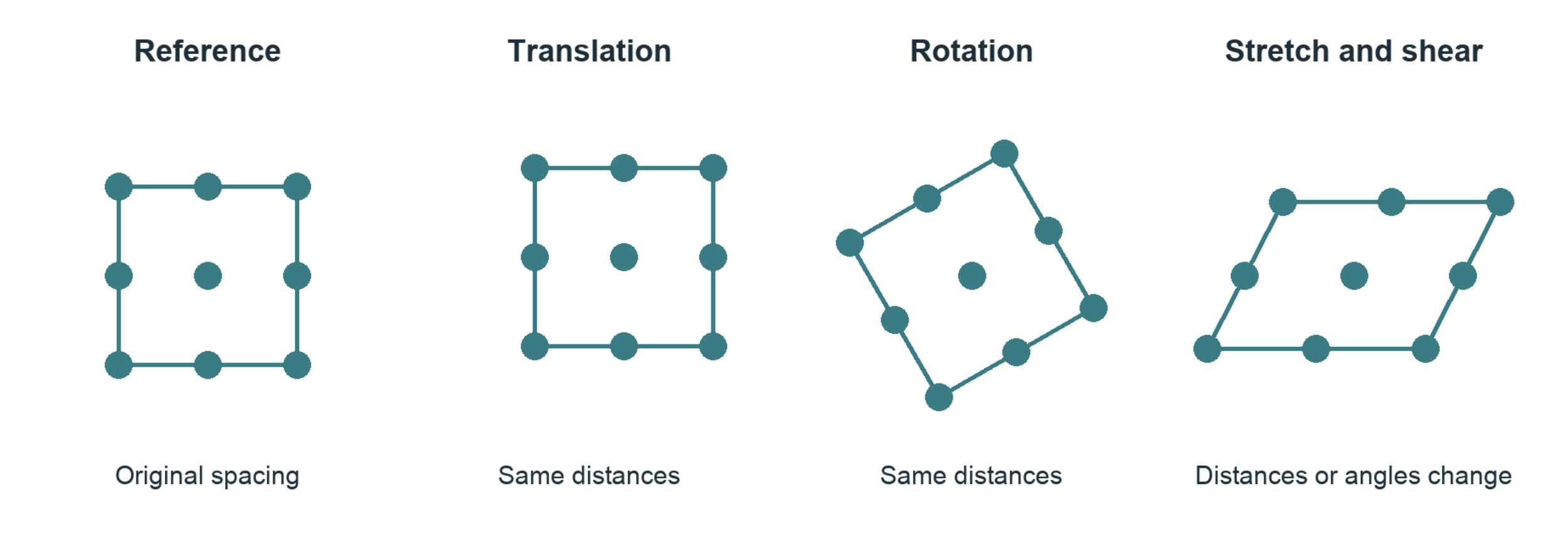
Translation and rigid rotation preserve shape. Stretch and shear alter the geometry. All four drawings use corresponding points.

Read this as: take the original position X, apply the transformation F, and add the translation t to obtain the new position x. In two dimensions F is a two-by-two matrix. Its first column tells us where a unit horizontal arrow goes; its second tells us where a unit vertical arrow goes. Every other arrow is built from those two.
For example, F with diagonal entries 1.05 and 1 stretches horizontal distances by 5 percent and leaves vertical distances unchanged. A 0.30 nm horizontal separation becomes 0.315 nm. Here nm means nanometer, one billionth of a meter.
Three meanings of transformation
A symmetry operation maps a whole pattern onto an indistinguishable version of itself.
A deformation maps a reference configuration into a changed configuration and may reduce its symmetry.
A Fourier transform, introduced later, changes the mathematical description of an image without moving any atoms.
Try it on paper. Draw four dots at the corners of a square. Translate them, rotate them, and then move the upper pair sideways. Which operations change a side length or an angle? That distinction is the beginning of strain measurement.
2 What ‘continuum’ means
Suppose we mark a flexible sheet with dots and gently stretch it. We can list the motion of each dot. We can also draw a smooth collection of arrows describing motion throughout the sheet, including positions between the dots. That collection of arrows is a displacement field.
A continuum description assigns quantities such as displacement or temperature throughout a region. It does not assert that atoms disappear or that matter has no gaps. It is a model whose spatial detail is chosen for the question being asked. Its usefulness must be tested at that scale.
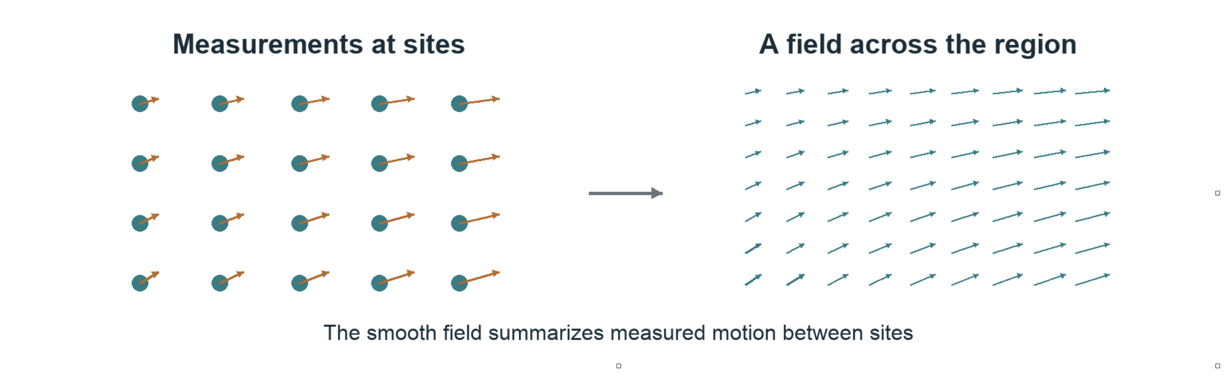
Discrete site measurements and a smooth field can describe the same deformation at different levels of detail. The arrows are schematic, not experimental results.

Displacement u is the arrow from an original position X to its current position x. The second expression says that, within a sufficiently small neighborhood, F transforms an original separation dX into a current separation dx. When F varies from place to place, each neighborhood has its own local transformation.
The local Cauchy Born idea
Aᵢ is a lattice separation before deformation and aᵢ is the corresponding separation afterward. The approximation asks whether one local continuum transformation also describes the lattice separations. Differences between measured aᵢ and predicted F Aᵢ are called non-affine residuals. They may reflect rearrangement, variation within the neighborhood, or measurement error.

For a motif containing several atoms, internal relative shifts may need extra variables. Near a defect, a single smooth transformation can become inadequate. Cauchy-Born is a relationship to test under stated conditions, not a guarantee supplied by drawing a smooth field [5].
3 Moiré turns small differences into readable signals
Place one fine line grating over another with a slightly different spacing. Broad dark and light bands appear. These moire bands record the changing alignment of the two fine patterns. A small difference at the carrier scale becomes a slow variation that is easier to inspect.
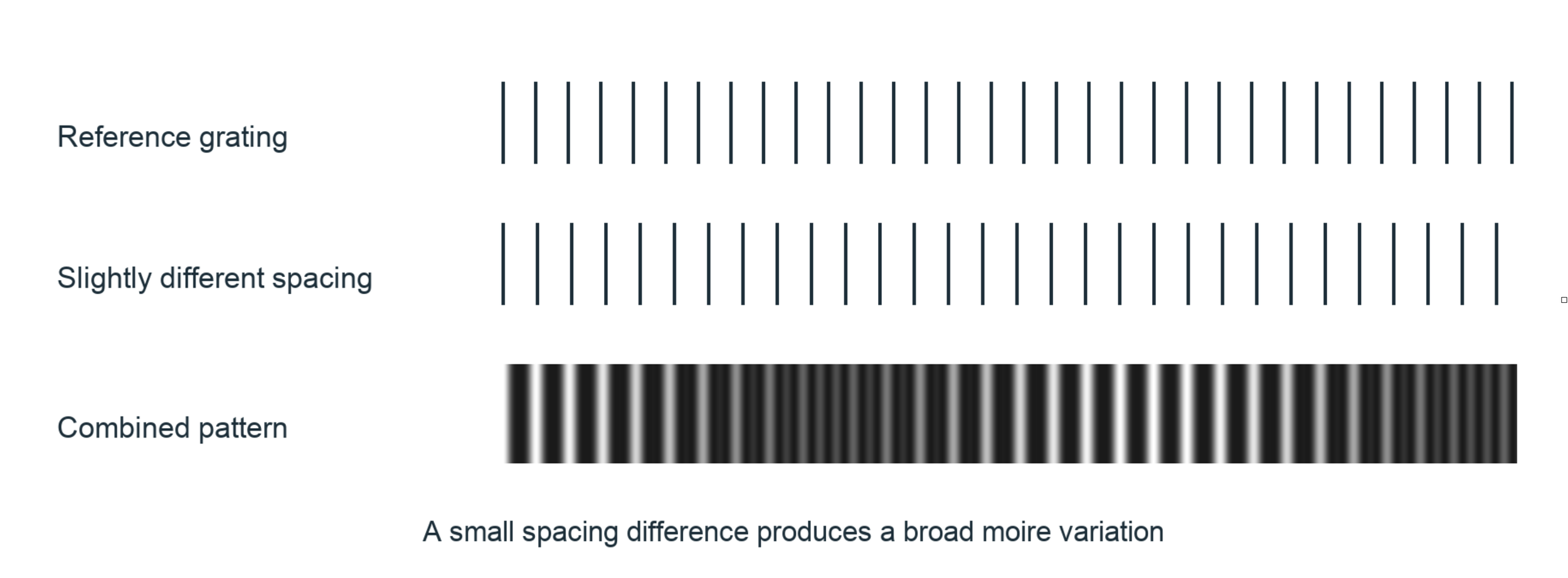
Two one-dimensional teaching gratings produce a broad difference pattern. Digital analysis can extract a phase difference without physically overlaying two gratings.
The carrier is the repeating pattern that carries displacement information. Its phase tells us where we are within one cycle: at a crest, halfway through, or somewhere between. One complete cycle is 2π radians. For a simple one-dimensional carrier we can write:

I is image intensity, A is background brightness, B is contrast, d is the carrier spacing, and u is a displacement along the carrier direction. Shifting the pattern shifts its phase. With the reference phase subtracted, this convention gives:

If d is 0.30 nm, a measured phase change of −0.02π radians corresponds to a positive displacement of 0.003 nm, or 3 picometers. This illustrates fractional-cycle sensitivity; it is not an accuracy claim for a microscope or for the software.
4 Reading an atomic image in frequency space
An atomic image contains many overlapping periodic features. A Fourier transform expresses the image as spatial frequencies: how often a pattern repeats and in what direction. A regular lattice produces pronounced peaks. Filtering around a selected peak isolates one family of lattice fringes [1, 4].
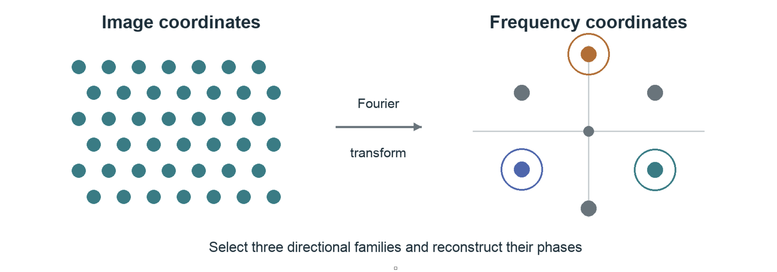
A schematic image and its reciprocal-space description. The circles select three example families. Peak positions encode repeat frequencies and directions, not the locations of individual atoms.
An inverse transform of one selected family produces a complex signal. Complex here means two numerical components that encode amplitude and phase. The phase is a computed description of the selected image carrier; it is not automatically the full electron-wave phase or an atomic electronic wavefunction.
Subtract a reference phase and the remaining phase records deviations from the chosen reference lattice. A reference may come from a separate image, an appropriate undistorted region, or a calibrated ideal carrier. That choice changes what displacement means and must be recorded.
The microscope remains part of the measurement
HRTEM intensity arises from electron scattering and the microscope optics. The contrast transfer function describes how spatial frequencies are transferred into image contrast under an applicable imaging approximation. Defocus and aberrations can weaken, reverse, or distort contrast. Thickness and crystal orientation also matter. A bright or dark spot is therefore not a direct electron-density reading [1, 4].
Digital moiré and holographic methods share the use of phase and references. The 2019 paper analyzes fringes extracted from HRTEM images; that is distinct from an off-axis electron-holography acquisition with a separate reference wave. No visible-light atomic-resolution claim follows from this analysis.
5 Three directions connect phase to motion
A single family of parallel fringes measures only the component of displacement normal to those fringes. Motion along them is invisible to that family. Combining families with different directions lets us recover a two-dimensional displacement vector.
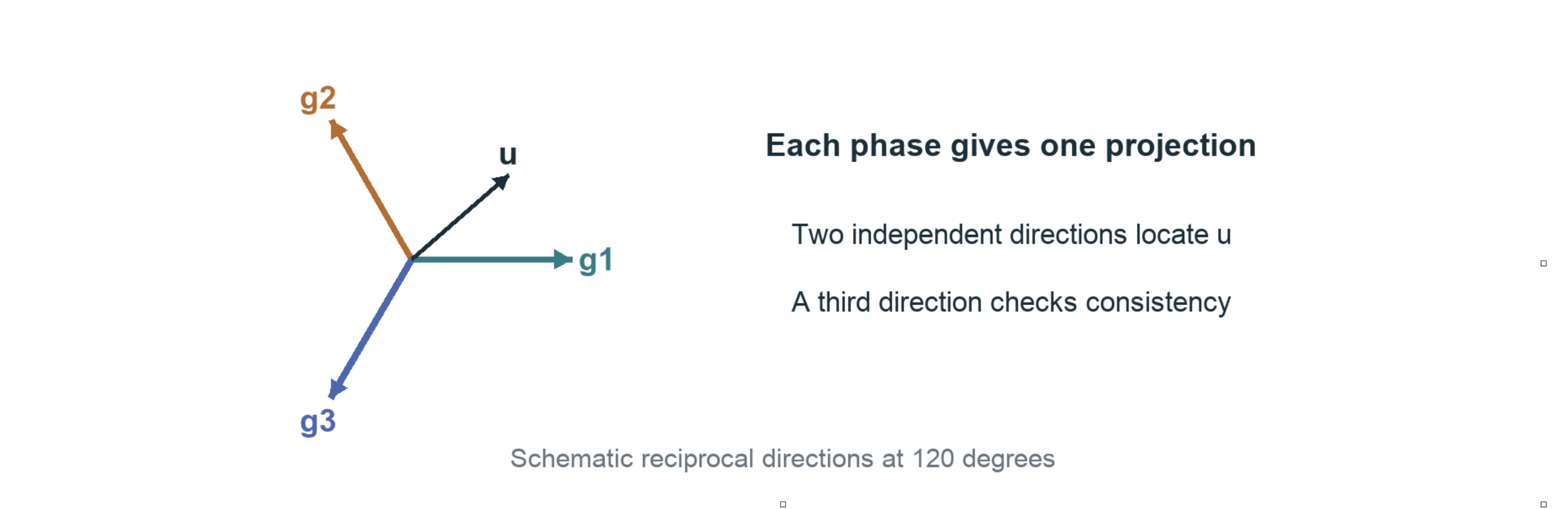
Each reciprocal vector g points normal to its carrier fringes. Its length is a spatial frequency. The three colored arrows are directions of measurement, not three independent spatial dimensions.

The dot means projection with scaling: gₖ · u = gₖₓuₓ + gₖᵧuᵧ. If g is measured in cycles per nanometer and u in nanometers, their product is a number of cycles. Multiplying by 2π gives radians. This sign assumes the positive Fourier order used in the Holomoire convention.
Two nonparallel directions can determine two displacement components. The third supplies redundancy and a consistency check. The paper uses the natural three-direction geometry of its hexagonal pattern, connecting it to a 120-degree strain rosette [1]. A rosette is a set of directional measurements combined to describe deformation.
The rosette also reads local changes of spacing

Here eₖ is a unit arrow along a specified measurement direction. J describes how displacement changes as we move through current spatial coordinates; sym(J) means its symmetric part. qₖ is a directional displacement derivative. Three suitable directions recover the three independent entries of this symmetric two-dimensional array.
These derivatives reveal stretching patterns, but sym(J) is not a finite-strain tensor for arbitrary rotation. Also, a direct-lattice vector and a reciprocal vector are different objects. Their directions and lengths must follow the calibrated crystal geometry, rather than being interchanged because both drawings look hexagonal.
6 Turning motion into strain
Move every atom by the same amount and the crystal translates without strain. Rotate the whole arrangement rigidly and it still has no strain. Strain concerns changes in the distances and angles between neighbors. This is why displacement alone is not enough: we need its local variation.
Two coordinate descriptions are useful. A material or Lagrangian description labels a point by its original position X. A spatial or Eulerian description labels it by its current position x. Neither choice by itself implies small deformation.

F is the deformation gradient, I is the identity transformation, and J is the spatial gradient of u(x) = x − X(x). The inverse reverses the mapping from current separations to reference separations. Two standard measures of finite strain are:

A strain tensor records how deformation depends on direction. E is Green-Lagrange strain, referred to the original configuration. e is Euler-Almansi strain, referred to the current configuration. The superscript T means transpose: exchange a matrix’s rows and columns. For a rigid rotation R, RᵀR = I, so both measures give zero.
The name of a strain measure matters
The paper also reports directional measures in equations 11–13. Their normal measures and angular shear measure differ from the standard tensor components above. For a uniaxial stretch ratio λ = 1.05, these definitions give:
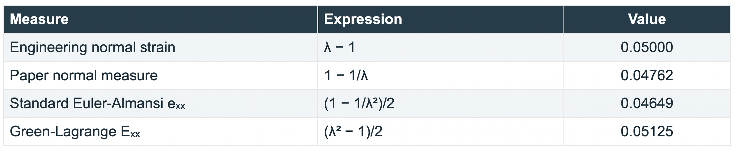
The four values describe the same prescribed stretch with different definitions. Principal strains describe the strain along special perpendicular directions without shear in that tensor representation. A strain ellipse is a geometrical description of deformed separations; it does not mean atomic nuclei become ellipses.
7 A dislocation interrupts the repeating pattern
In a simple cross-section, an edge dislocation can be pictured as the termination of an extra atomic half-plane. Neighboring positions rearrange around that termination. The usual elastic picture has compression on the crowded side and tension on the opposite side, with directions set by the defect orientation.
The arrangement remains ordered over much of the image, but the reference lattice cannot be continued around the defect without a mismatch. That mismatch is described by a Burgers vector. It records the lattice translation associated with going around the defect.
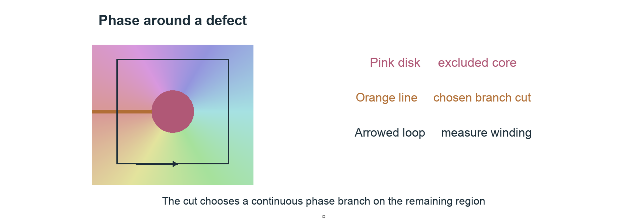
A schematic phase winding, with the core and one chosen cut. This is a topological illustration, not a calculated SiC strain field or an image of a physical crack.

Φₖ is the total phase change accumulated around a counterclockwise loop. Add the small changes along the loop, preserving the full cycles. nₖ is the signed number of cycles; b is the Burgers vector defined by the corresponding displacement increment. The equation uses our earlier phase sign. Other closing-vector conventions can reverse the sign.
Phase is normally reported modulo 2π, just as a clock face repeats after one turn. Unwrapping chooses continuous values by counting turns. Around a dislocation, a single continuous branch cannot cover a loop enclosing the singularity. A branch cut selects a route from the core to a boundary across which we allow the branch to jump.
The line and the center spot. The displayed cut is a mathematical choice, not a predicted crack. The core mask marks a region excluded from reliable reconstruction. Strain fits must not bridge either exclusion. Moving a valid cut can change displacement by a lattice period on part of the image while leaving local deformation away from the cut unchanged.
8 What the SiC paper contributes
The paper treats the crystal pattern as an experimental carrier of deformation information. It connects measurements of selected elementary cells to phase-derived fields around dislocations in 4H-SiC. Its distinctive emphasis is the connection between the crystallographic rosette, continuum kinematics, and the local arrangement of the crystal [1].
These are two related ways to read the same experimental geometry: inspect how a cell changes, and inspect how displacement varies across the field. Their agreement supports the usefulness of a continuum description in the regions and conditions examined. Because they share image information, agreement is not a fully independent experimental test.
Geometry supplies evidence about interactions
Atomic interactions govern which arrangements are stable and how a material responds to loading. Measuring the resulting arrangement gives us evidence against which an interaction model can be tested. Displacement and strain alone do not uniquely identify bonding energies, interatomic forces, or electron density.

This is a one-dimensional linear elastic example. Stress σ describes internal force per area. Strain ε describes deformation. Young’s modulus Y supplies a material relationship between them. The paper estimates stresses using elastic constants and a plane-stress assumption. Those stresses depend on the adopted material model; they are not directly read from image brightness.
The authors describe their observations as proving Cauchy-Born within the observed range. A cautious scientific reading is that they provide experimental support for a kinematic correspondence. A general claim would require independent data, uncertainty estimates, and tests of where that correspondence fails. Conditional mathematical results already existed [5].
Fourier-phase strain mapping also predates this paper [4]. The 2019 work is valuable as a particular experimental-mechanics treatment of the atomic-to-continuum connection. The paper explicitly leaves force-driven dynamics outside its scope.
10 Holomoire SiC Sim Library
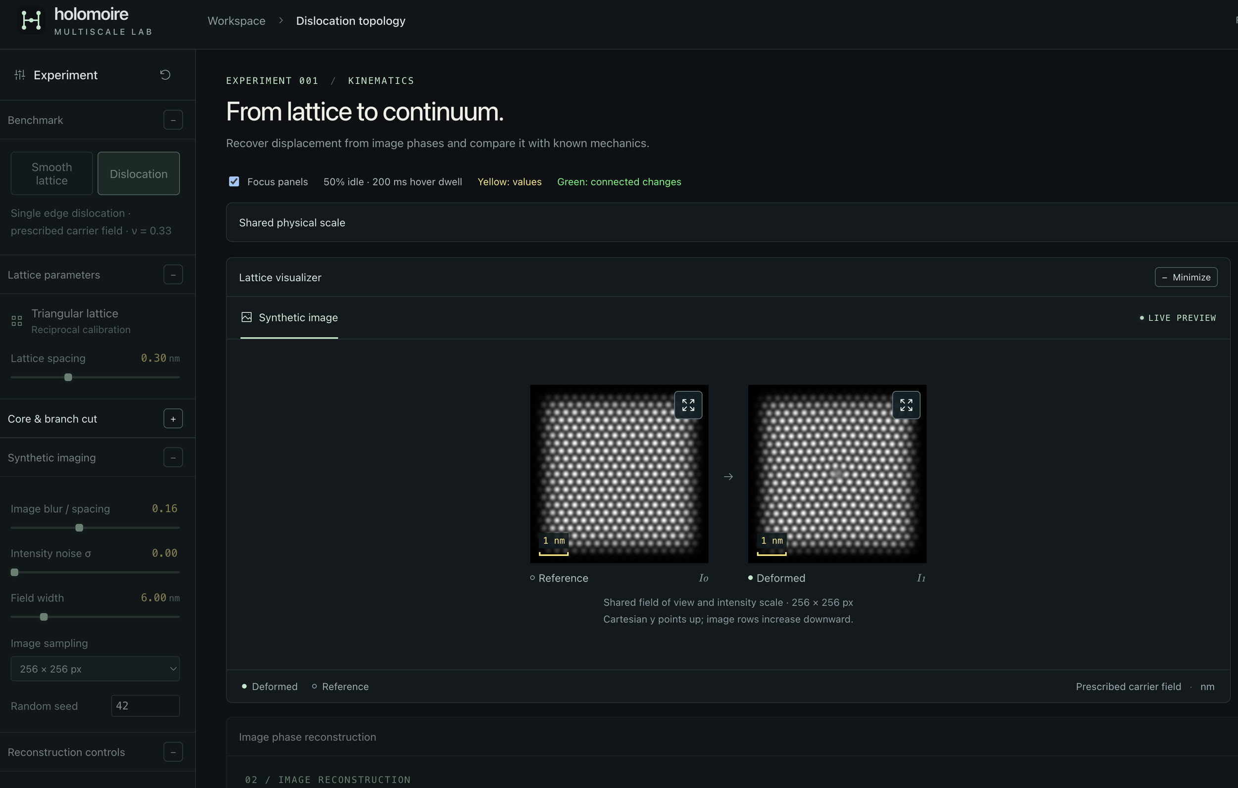
The Holomoire SiC Sim Library is our developing collection of computational tools for exploring this measurement chain. Its current browser workbench lets a student prescribe a pattern change, generate an image, reconstruct displacement from that image, and compare the reconstruction with the prescribed answer. Reusable Python functions perform the scientific calculations.
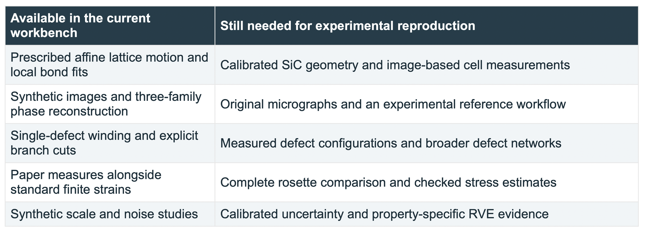
The library connects the objects introduced in this guide: motifs and lattice geometry, transformations, directional carriers, phase, displacement, strain, and analysis scale. Its present synthetic lattice is illustrative. The SiC name identifies the research direction; the current release is not a calibrated 4H-SiC simulator or a completed reproduction of the paper.
Three first experiments
1. Translate and rotate. Compare the zero strain from exact bond geometry with the small errors in image-derived strain. Change the translation anchor to see why periodic images leave lattice-period ambiguity.
2. Stretch and recover. Prescribe a small stretch, reconstruct it from the image, and compare the recovered field with the known field. Increase noise or change the Fourier bandwidth. Read the error together with the valid area.
3. Inspect a dislocation. Follow the directional phases around the core and move the branch cut. Compare local strain away from exclusions, then disable the cut to see why the solver refuses an unresolved singular domain.
Sources for further study
[1] C. A. Sciammarella, F. M. Sciammarella, and L. Lamberti. Determination of Displacement Fields at the Sub-Nanometric Scale. Materials 12, 1804 (2019). Primary scientific reference. Read source
[2] B. Wuensch. Introduction to Crystallography Part 1. MIT OpenCourseWare, 3.60, Fall 2005. A geometry-led introduction to patterns and transformations. Read source
[3] B. Wuensch. Translation Rotation Periodicity Part 1. MIT OpenCourseWare, 3.60, Fall 2005. Translation, motifs, and the distinction between lattice points and atoms. Read source
[4] M. J. Hytch, E. Snoeck, and R. Kilaas. Quantitative measurement of displacement and strain fields from HREM micrographs. Ultramicroscopy 74, 131–146 (1998). Fourier-phase reconstruction and imaging limitations. Read source
[5] W. E and P. Ming. Cauchy-Born Rule and the Stability of Crystalline Solids: Static Problems. Archive for Rational Mechanics and Analysis 183, 241–297 (2007). Conditional mathematical connection between atomistic and continuum elasticity. Read source